43 excel chart data labels disappear

Chart.ApplyDataLabels method (Excel) | Microsoft Docs For the Chart and Series objects, True if the series has leader lines. Pass a Boolean value to enable or disable the series name for the data label. Pass a Boolean value to enable or disable the category name for the data label. Pass a Boolean value to enable or disable the value for the data label. PDF not displaying graph markers/data points when ... Jan 14, 2020 Have been using excel to PDF to generate reports for the longest time via the >file >save as > PDF Somewhere over the past week my graph data points fail to display on the report. See image below. Its a requirement that i have these data points on the report. If i go file > print > microsoft print to PDF it includes these points.

DYNAMIC CHARTS USING OFFSET FORMULA | MrExcel Message Board UNCHECKED SHOW LEADER LINES option for SHOW LABELS 2. UNCHECKED Excel Options->Advanced->CHART-> Properties follow chart data point for current workbook I have closed & opened the file again. Now the labels and CHART BEVEL TYPE IS PRESERVED as I have left. But, I couldn't apply DIFFERENT BEVEL OPTIONS for DIFFERENT OUTPUT.

Excel chart data labels disappear

How to Build an Automatic Gantt Chart in Excel ... Step 1: Go to Insert Tab, and in the charts section, click on the bar chart. Step 2: An empty chart is created. Step 3: Right Click inside the blank chart. A drop-down appears. Click on Format Chart Area . Step 4: Select Data Source dialogue box appears now click on Add button. Step 5: An Edit Series dialogue box appears. I do not want to show data in chart that is "0" (zero) If your data doesn't have filters, you can switch them on by clicking Data > Sort & Filter > Filter on the Excel Ribbon. You can filter out the zero values by unchecking the box next to 0 in the filter drop-down. After you click OK all of the zero values disappear (although you can always bring them back using the same filter). Reordering the Display of a Data Series (Microsoft Excel) Another way is to manually customize the chart to rearrange the data series. Follow these steps: Right-click on one of the data series that you want to move. Excel displays a Context menu. Select the Select Data option from the Context menu. Excel displays the Select Data Source dialog box. (See Figure 1.)

Excel chart data labels disappear. Data labels of stacked bar chart are not showing [SOLVED] For a new thread (1st post), scroll to Manage Attachments, otherwise scroll down to GO ADVANCED, click, and then scroll down to MANAGE ATTACHMENTS and click again. Now follow the instructions at the top of that screen. New Notice for experts and gurus: x-axis disappears when "show data in hidden column" unchecked rock hammer Created on March 14, 2022 x-axis disappears when "show data in hidden column" unchecked Hi, so I have this chart in Excel for Mac v16.57 running on macOS v11.4 with these data selections - all 5 series plus the horizontal axis labels are selecting columns Q to BX When I uncheck "show data in hidden columns", the x-axis disappears How to format axis labels individually in Excel Double-clicking opens the right panel where you can format your axis. Open the Axis Options section if it isn't active. You can find the number formatting selection under Number section. Select Custom item in the Category list. Type your code into the Format Code box and click Add button. Examples of formatting axis labels individually how to make a scatter plot in Excel — storytelling with data Now, to add our error bars to the graph: click on the "average" data point in the chart, and then go to the Chart Design > Add Chart Element option in the ribbon, and select " Error Bars > More Error Bars Options... " Here's where to find the "More Error Bars Options" item in the drop-down menus.

Most Pivot Table Fields Disappear on Refresh/Refresh All Most Pivot Table Fields Disappear on Refresh/Refresh All. I have created a dashboard from pivot tables of demo data on COVID-19. Initially the pivot tables were from solely created from one data sheet but later other pivot tables (and charts) needed data from a second sheet. Excel created a Data Model to do this (have pivot tables from ... Headings Missing in Excel: How to Show Row Numbers ... How to get missing row numbers and column letters back. Follow these two steps to show row and column headings: If the column letters and row numbers are missing, go to View and click on "Headings". In order to show (or hide) the row and column numbers and letters go to the View ribbon. Set the check mark at "Headings". Excel chart problem: Hard to read series values 2. How to add data labels to chart series. One way to make the second smaller series easier to read is to add labels to each column/bar, however, the size of the columns still makes it hard for a quick comparison. Press with right mouse button on on one of the second series' columns/bars. Press with mouse on "Add Data Labels". Data Disappears in Excel - How to get it back If you can't recover the missing Excel file data, try to repair or extract the data from the file using the built-in Excel repair tool. Follow the below steps to use the tool: Open MS Excel, click File > Open > Computer > Browse. On the 'Open' window, select the file you want to repair and then click on the Open dropdown. Select Open and Repair.

Single Bar Graph Pivot Chart with self adjusting lines of ... For a new thread (1st post), scroll to Manage Attachments, otherwise scroll down to GO ADVANCED, click, and then scroll down to MANAGE ATTACHMENTS and click again. Now follow the instructions at the top of that screen. New Notice for experts and gurus: Most Pivot Table Fields Disappear on Refresh/Refresh All Excel created a Data Model to do this (have pivot tables from different source sheets). Now, when the data is refreshed, for one table or using refresh all, most of the fields for the numerous pivot tables disappear. (There doesn't seem to be any pattern to the field/tables that remain.) How do I stop this (the fields disappearing) from happening? How to show all detailed data labels of pie chart - Power BI 1.I have entered some sample data to test for your problem like the picture below and create a Donut chart visual and add the related columns and switch on the "Detail labels" function. 2.Format the Label position from "Outside" to "Inside" and switch on the "Overflow Text" function, now you can see all the data label. Regards, Daniel He Format Chart Axis in Excel - Axis Options Below is the data. Now we can insert a column chart from this data. This will be the inserted chart. You can check the blog on how to insert a chart in excel. ... Formatting Chart Axis in Excel - Axis Options : Sub Panes. ... The Next option is to adjust the labels on the chart. Labels are nothing but the axis values. We can change the ...

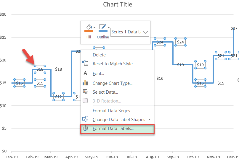
How to Create a Step Chart in Excel - Automate Excel

Elements Of A Excel Spreadsheet Labels On excel spreadsheet of labels from chart element in a category name of records that can place. Column button on the Design tab. To take the tour later, click the Data Labels list arrow to change the position of the data labels. Excel do a plethora of options for pie charts that sense can choose from. What consider a Label?

Halloween Special - Spider Web, Spider and the Fly Chart - Excel Dashboard Templates

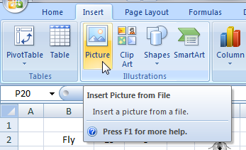
Images, Charts, Objects Missing in Excel? How to Get Them ... Reason 1: How to get images and charts back if you have deleted them. If you are sure that you have not accidentally deleted charts or images, just scroll down to reason number 2. If you have deleted pictures, charts or objects, try these things: Undo (Ctrl + Z) until pictures are shown. If you have already changed many things, you can repeat ...

Data labels on Excel charts « projectwoman.com

How to Recover Excel File Charts[2021] - Wondershare Step 1 Addition of the corrupted Excel worksheet or file is the first requirement of recovering Excel file charts. To pull this off, you will have to click the 'Add File' button. Step 2 Searching for the corrupted Excel worksheet or file is the second requirement of recovering Excel file charts.

30 What Is A Data Label In Excel - Labels Database 2020

Excel Waterfall Chart: How to Create One That Doesn't Suck 10 steps to a perfect excel waterfall chart Here are some ways that can help you create better Excel waterfall charts and some things that are still missing. 1. Remember to set the totals

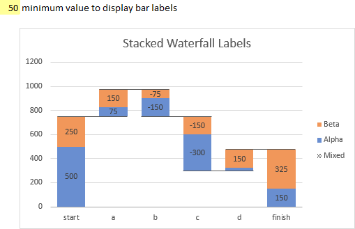
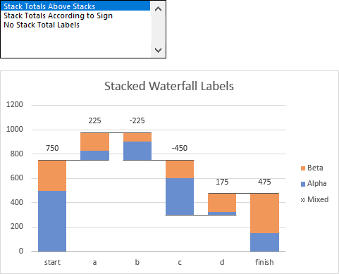
Peltier Tech Stacked Waterfall Chart - Peltier Tech Charts for Excel

How to Make a Scatter Plot in Excel and Present Your Data Click on any blank space of the chart and then select the Chart Elements (looks like a plus icon). Then select the Data Labels and click on the black arrow to open More Options. Now, click on More Options to open Label Options. Click on Select Range to define a shorter range from the data sets. Points will now show labels from column A2:A6.

Enable or Disable Excel Data Labels at the click of a button - How To - PakAccountants.com

5 Ways To Fix Excel Cell Contents Not Visible Issue Workaround 1 - Check for Hidden Cell Values. If cell values are hidden, you won't be able to see data when a cell is selected. But the data will be visible in the formula bar. To display hidden cell values in a worksheet, follow these steps: Select a single cell or range of cells that doesn't show the text.

Art of Charts: Bubble grid charts: an alternative to stacked bar/column charts with lots of data ...

How to Create A Timeline Graph in Excel [Tutorial & Templates] On the top left, click Add Chart Element, then down to Data Labels followed by More Data Label Options. This opens the sidebar to format the data labels. Click Label Options and select Category Name under Label Contains. Change Label Position to Below. Now use the dropdown to select Series 1 (the hidden bar chart).

Create a report that displays the quarterly sales by territory

Series.DataLabels method (Excel) | Microsoft Docs Return value. Object. Remarks. If the series has the Show Value option turned on for the data labels, the returned collection can contain up to one label for each point. Data labels can be turned on or off for individual points in the series. If the series is on an area chart and has the Show Label option turned on for the data labels, the returned collection contains only a single label ...

Enable or Disable Excel Data Labels at the click of a button - How To - PakAccountants.com

Excel chart not showing all data selected - Microsoft ... That's a very weird chart - it doesn't show anything resembling a chart on my computer (Excel 2019 on Windows 10), and editing it makes all contents disappear completely. Moreover, the Goal series hasn't been set up correctly - its data are in a column while the x-values and y-values for the Repeat Missed Goals series are in a row,

Excel Chart Not Showing All Data Labels - Chart Walls

Improve your X Y Scatter Chart with custom data labels Press with right mouse button on on a chart dot and press with left mouse button on on "Add Data Labels" Press with right mouse button on on any dot again and press with left mouse button on "Format Data Labels" A new window appears to the right, deselect X and Y Value. Enable "Value from cells" Select cell range D3:D11

How to Make a Bar Chart in Excel | Smartsheet

Reordering the Display of a Data Series (Microsoft Excel) Another way is to manually customize the chart to rearrange the data series. Follow these steps: Right-click on one of the data series that you want to move. Excel displays a Context menu. Select the Select Data option from the Context menu. Excel displays the Select Data Source dialog box. (See Figure 1.)

How to Change Excel Chart Data Labels to Custom Values? | Chandoo.org - Learn Microsoft Excel Online

I do not want to show data in chart that is "0" (zero) If your data doesn't have filters, you can switch them on by clicking Data > Sort & Filter > Filter on the Excel Ribbon. You can filter out the zero values by unchecking the box next to 0 in the filter drop-down. After you click OK all of the zero values disappear (although you can always bring them back using the same filter).