39 excel chart data labels outside end
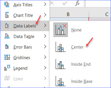
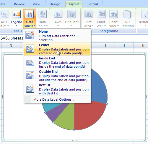
peltiertech.com › broken-y-axis-inBroken Y Axis in an Excel Chart - Peltier Tech Nov 18, 2011 · For the many people who do want to create a split y-axis chart in Excel see this example. Jon – I know I won’t persuade you, but my reason for wanting a broken y-axis chart was to show 4 data series in a line chart which represented the weight of four people on a diet. One person was significantly heavier than the other three. How to: Display and Format Data Labels - DevExpress To specify the location of data labels on the chart, use the DataLabelBase.LabelPosition property. In this example, the DataLabelPosition.Center value is used, so data labels will be displayed centered inside columns. View Example DataLabelsActions.cs DataLabelsActions.vb
Date Axis in Excel Chart is wrong • AuditExcel.co.za How to force Excel to use your typed in dates in a chart Although this feature is useful, sometimes you just want Excel to show the dates you typed. In order to do this you just need to force the horizontal axis to treat the values as text by right clicking on the horizontal axis, choose Format Axis Change Axis Type to be Text

Excel chart data labels outside end
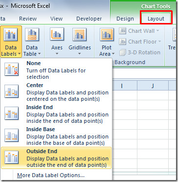
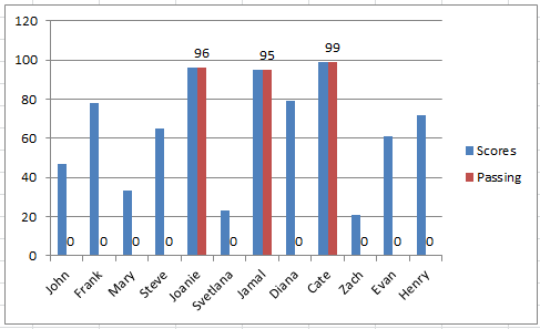
Controlling Chart Gridlines (Microsoft Excel) - ExcelTips (ribbon) Select the chart by clicking on it. You should see selection handles appear around the outside of the chart. Make sure that the Layout tab of the ribbon is displayed. (This tab is only visible when you've selected the chart in step 1.) Click the Gridlines tool in the Axes group. You'll see a drop-down menu appear with various options. How to denote letters to mark significant differences in a bar chart ... 1) Select cells A2:B5 2) Select "Insert" 3) Select the desired "Column" type graph 4) Click on the graph to make sure it is selected, then select "Layout" 5) Select "Data Labels" ("Outside End" was... What does the "@" symbol mean in Excel formula (outside a table) How is it used The @ symbol is already used in table references to indicate implicit intersection. Consider the following formula in a table = [@Column1]. Here the @ indicates that the formula should use implicit intersection to retrieve the value on the same row from [Column1].
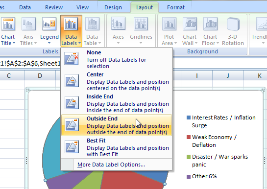
Excel chart data labels outside end. Excel x axis not showing last value - Profit claims 2. Click on the "Layout" tab at the top of the Excel window, then click the drop-down arrow on the left side of the ribbon and choose "Horizontal (Category) Axis" from the list of options. Click the "Format Selection" button next to the drop-down arrow to continue. The Format Axis window appears. Stacked Bar Chart in Power BI [With 27 Real Examples] Initially, make sure the data source has been loaded to the Power BI report canvas and select the Stacked bar chart and add it to the report canvas as shown below: X-axis - Profit and Sales Y-axis - Product Power BI stacked bar chart Multiple axes Make Excel charts primary and secondary axis the same scale The problem is you need to go into the chart every time the data changes. Create a common scale for the Primary and Secondary axis. The trick is to create a common scale so that the primary and secondary axis start and end at the same point. The only way this can happen is if the smallest and biggest number for both data series are the same. MsoChartElementType enumeration (Office) | Microsoft Learn Display data label inside at the base. msoElementDataLabelInsideEnd: 203: Display data label inside at the end. msoElementDataLabelLeft: 206: Display data label to the left. msoElementDataLabelNone: 200: Do not display data label. msoElementDataLabelOutSideEnd: 205: Display data label outside at the end. msoElementDataLabelRight: 207: Display ...
superuser.com › questions › 1285179microsoft excel - Adding data label only to the last value ... Jan 13, 2018 · In your case, after Label is applied, Right Click the Line, you find Labels are ready to Edit. Select Labels one by one, then either Right Click & Delete or un-check the Value Checkbox next to the Chart Area. VBA Solution: Create one Command button and enter this code. Remember, you simply create the Chart but don't apply the Data Labels. Data Labels bar chart - inside end if negative and outside end if ... (A stacked column chart has the overlap set to 100% by default, but it doesn't allow outside end data labels.) I added my data labels, and positioned them outside or inside end. If you want the bars to look the same, you can apply the same color to both sets. You must log in or register to reply here. Custom Chart Data Labels In Excel With Formulas - How To Excel At Excel Follow the steps below to create the custom data labels. Select the chart label you want to change. In the formula-bar hit = (equals), select the cell reference containing your chart label's data. In this case, the first label is in cell E2. Finally, repeat for all your chart laebls. support.microsoft.com › en-us › officeUpdate the data in an existing chart - support.microsoft.com Show or hide a chart legend or data table Article; Add or remove a secondary axis in a chart in Excel Article; Add a trend or moving average line to a chart Article; Choose your chart using Quick Analysis Article; Update the data in an existing chart Article; Use sparklines to show data trends Article
› how-to-make-charts-in-excelHow to Make Charts and Graphs in Excel | Smartsheet Jan 22, 2018 · To generate a chart or graph in Excel, you must first provide the program with the data you want to display. Follow the steps below to learn how to chart data in Excel 2016. Step 1: Enter Data into a Worksheet. Open Excel and select New Workbook. Enter the data you want to use to create a graph or chart. spreadsheeto.com › bar-chartHow To Make A Bar Graph in Excel - Spreadsheeto Here are three things that make bar charts a go-to chart type: 1. They’re easy to make. When your data is straightforward, designing and customizing a bar chart is as simple as clicking a few buttons. There aren’t many options, you don’t need to organize your data in a complicated way, and Excel is good at extracting your headings and ... peltiertech.com › add-horizontal-line-to-excel-chartAdd a Horizontal Line to an Excel Chart - Peltier Tech Sep 11, 2018 · This tutorial shows how to add horizontal lines to several common types of Excel chart. We won’t even talk about trying to draw lines using the items on the Shapes menu. Since they are drawn freehand (or free-mouse), they aren’t positioned accurately. Since they are independent of the chart’s data, they may not move when the data changes. DataLabels.Separator property (Excel) | Microsoft Learn If you use xlDataLabelSeparatorDefault (= 1) ( XlDataLabelSeparator enumeration), you'll get the default data label separator, which is either a comma or a newline, depending on the data label. When a value of "1" is returned, it indicates that the user has not changed the default separator, which is a comma ",".
How to Change Data Labels in Excel (with Easy Steps) - ExcelDemy
How to wrap text in Excel automatically and manually - Ablebits.com Method 1. Go to the Home tab > Alignment group, and click the Wrap Text button: Method 2. Press Ctrl + 1 to open the Format Cells dialog (or right-click the selected cells and then click Format Cells… ), switch to the Alignment tab, select the Wrap Text checkbox, and click OK. Compared to the first method, this one takes a couple of extra ...

Change the format of data labels in a chart
Excel Waterfall Chart: How to Create One That Doesn't Suck - Zebra BI Ideally, you would create a waterfall chart the same way as any other Excel chart: (1) click inside the data table, (2) click in the ribbon on the chart you want to insert. ... in Excel 2016 Microsoft decided to listen to user feedback and introduced 6 highly requested charts in Excel 2016, including a built-in Excel waterfall chart.

How to Use Cell Values for Excel Chart Labels
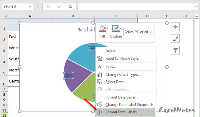
How to Edit Pie Chart in Excel (All Possible Modifications) This will create a new ribbon named Format Chart Area at the right side of the Excel file. Subsequently, go to the Chart Options menu >> Fill & Line icon >> Border group. Now, choose what type of border line you want. If you want a solid line border, choose the option Solid line. From the Color option, you can fix the border color.

6ExcelFig6 - Strategic Finance
Pie of Pie Chart in Excel - Inserting, Customizing - Excel Unlocked This is going to open a Format Data Labels pane at the right of excel. Mark the percentage, category name, and legend key. Select the position of data labels at Outside End. Select the fill color for data labels as white as we will change the chart background in the coming section. You can do it from the fill tab of the opened pane.
How to make data labels really outside end? - Microsoft Power ...
How to change Layout and Chart Style in Excel Layout 10: Layout 10 shows the following chart elements: Chart Title, Legend (Right), Data Labels (Outside End), Horizontal Axis, Vertical Axis, and Major Gridlines.. Layout 11: Layout 11 shows ...
How to Add Data Labels to a Chart - ExcelNotes
How to Create A Timeline Graph in Excel [Tutorial & Templates] - Preceden Go to Label Options and then change Label Contains to Category Name only. Change the Label Position to Outside End. Now select the horizontal axis on the chart and hit delete on the keyboard. You should now see your actions as labels at the end of the lines touching the horizontal line. The dates will show below the horizontal line.

Optimally positioning pie chart data labels in Excel with VBA ...
How to stop text spilling over in Excel - Ablebits.com Select the cells you wish to stop from spilling over. On the Home tab, in the Cells group, click Format > Row Height . The Row Height box will appear showing the current height of the selected cells. Click OK without changing anything just to confirm your present row height.
How-to Make a WSJ Excel Pie Chart with Labels Both Inside and ...
Excel tutorial: build a dynamic bump chart of the English Premier League Select the line in the chart menu: Format > then the drop down menu of chart elements > select the very last team name series (not the data labels). Hit Ctrl + 1 to bring up the formatting menu and change the line format (dark red + 2pt + large markers). 15. Format the dynamic line data labels. This is a little tricky.
Add Labels with Lines in an Excel Pie Chart (with Easy Steps)
How to add a single vertical bar to a Microsoft Excel line chart In the Chart Layouts group, click Add Chart Element. From the dropdown, choose Axes. From the resulting submenu, choose Secondary Vertical ( Figure J ), which displays the axes values to the right...

How to Make Pie Chart with Labels both Inside and Outside ...
How can I get data labels to show for each column in a bar chart? Turn on 'Overflow text' under Data label' Format tab. Also, you can adjust the position of the Data Label by switching to 'Outside End' or 'Inside Center' so that your Data Label gets displayed properly. If this post helps, then mark it as 'Accept as Solution ' so that it could help others. Regards, Sanket Bhagwat View solution in original post

Add Labels ON Your Bars
Waterfall charts with Excel, Matplotlib and Plotly I also selected patches and labels manually to define each color. plt.figure (figsize = (6, 6)) colors = ["royalblue","green","green","red","red","red", "royalblue", "red", "red", "red", "royalblue"] fig = df.T [1:].max (axis = 1).plot (kind = "bar", bottom = df ["Base"], width = 0.8,

Google Workspace Updates: Get more control over chart data ...
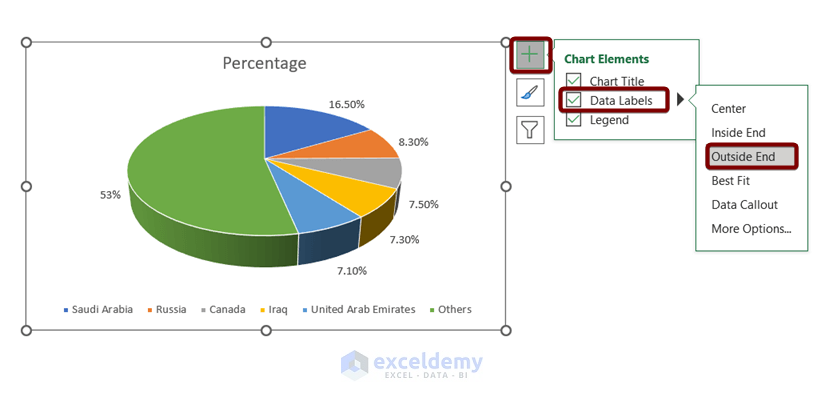
Pie Chart in Excel - Inserting, Formatting, Filters, Data Labels Right click on the Data Labels on the chart. Click on Format Data Labels option. Consequently, this will open up the Format Data Labels pane on the right of the excel worksheet. Mark the Category Name, Percentage and Legend Key. Also mark the labels position at Outside End. This is how the chark looks. Formatting the Chart Background, Chart Styles

How To Show Or Hide Data Labels On MS Excel? | My Windows Hub
Excel Conditional Formatting Data Bars - Contextures Excel Tips On the Ribbon, click the Home tab. In the Styles group, click Conditional Formatting, and then click Manage Rules. In the list of rules, click your Data Bar rule. Click the Edit Rule button, to open the Edit Formatting Rule dialog box. In the second section -- Edit the Rule Description -- add a check mark to Show Bar Only.
Format Data Label: Label Position - Microsoft Community
How to Make a Graph in Excel (2022 Guide) | ClickUp Select the Excel Chart Title > double click on the title box > type in "Movie Ticket Sales.". Then click anywhere on the excel sheet to save it. Note: you can also add other graph elements such as Axis Title, Data Label, Data Table, etc., with the Add Chart Element option. You'll find it under the Chart Design tab.

How to make doughnut chart with outside end labels - Simple ...
Unlink Chart Data - Peltier Tech It's easy to link many of a chart's text elements to a worksheet range. Select the text element, click in the formula bar, type = and click on the cell or range containing the text you want displayed. The result is a link formula like =Sheet1!$A$1, and the text element updates dynamically to display whatever is in the reference.

Create a column chart with percentage change in Excel
Adding Data Labels to Your Chart (Microsoft Excel) - ExcelTips (ribbon) To add data labels in Excel 2013 or later versions, follow these steps: Activate the chart by clicking on it, if necessary. Make sure the Design tab of the ribbon is displayed. (This will appear when the chart is selected.) Click the Add Chart Element drop-down list. Select the Data Labels tool.

Stagger long axis labels and make one label stand out in an ...
stackoverflow.com › questions › 48559387stacked column chart for two data sets - Excel - Stack Overflow Feb 01, 2018 · I wonder if there is some way (also using VBA, if needed) to create a stacked column chart displaying two different data sets in MS Excel 2016. Looking around, I saw the same question received a positive answer when working with Google Charts (here's the thread stacked column chart for two data sets - Google Charts )
Outside End Labels - Microsoft Community
What does the "@" symbol mean in Excel formula (outside a table) How is it used The @ symbol is already used in table references to indicate implicit intersection. Consider the following formula in a table = [@Column1]. Here the @ indicates that the formula should use implicit intersection to retrieve the value on the same row from [Column1].

Chart Data Labels in PowerPoint 2013 for Windows
How to denote letters to mark significant differences in a bar chart ... 1) Select cells A2:B5 2) Select "Insert" 3) Select the desired "Column" type graph 4) Click on the graph to make sure it is selected, then select "Layout" 5) Select "Data Labels" ("Outside End" was...
Stagger long axis labels and make one label stand out in an ...
Controlling Chart Gridlines (Microsoft Excel) - ExcelTips (ribbon) Select the chart by clicking on it. You should see selection handles appear around the outside of the chart. Make sure that the Layout tab of the ribbon is displayed. (This tab is only visible when you've selected the chart in step 1.) Click the Gridlines tool in the Axes group. You'll see a drop-down menu appear with various options.

How to Make Pie Chart with Labels both Inside and Outside ...

Add or remove data labels in a chart

Outside End Labels - Microsoft Community

Enable or Disable Excel Data Labels at the click of a button ...
microsoft excel - How do I reposition data labels with a ...

How to show data labels in PowerPoint and place them ...
Excel 2010: Show Data Labels In Chart
How to Make Pie Chart with Labels both Inside and Outside ...
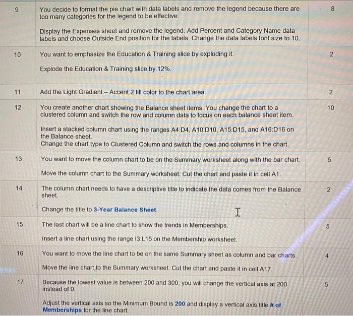
Step Instructions Points Possible 1 1 0 Start Excel. | Chegg.com

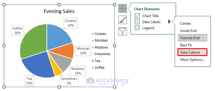
Add data labels and callouts to charts in Excel 365 ...

How to Make a Bar Graph in Excel (Clustered & Stacked Charts)
What Are Data Labels in Excel (Uses & Modifications)
How-to Make a WSJ Excel Pie Chart with Labels Both Inside and ...

How to Make a Graph in Excel - All Things How

Add or remove data labels in a chart
Move and Align Chart Titles, Labels, Legends with the Arrow ...
Add Data Labels Outside End for Dynamic Label Threshold Chart ...

Is there a way to add data labels as percentages on the ...

How to make doughnut chart with outside end labels - Simple ...
Post a Comment for "39 excel chart data labels outside end"