45 adding chart labels in excel

› charts › gauge-templateExcel Gauge Chart Template - Free Download - How to Create Step #11: Add the chart title and labels. You’ve finally made it to the last step. A gas gauge chart without any labels has no practical value, so let’s change that. Follow the steps below: Go to the Format tab. In the Current Selection group, click the dropdown menu and choose Series 1. This step is key! Tap the menu key on your keyboard ... how to add data labels into Excel graphs Feb 10, 2021 ... Right-click on a point and choose Add Data Label. You can choose any point to add a label—I'm strategically choosing the endpoint because that's ...

chandoo.org › wp › change-data-labels-in-chartsHow to Change Excel Chart Data Labels to Custom Values? May 05, 2010 · The Chart I have created (type thin line with tick markers) WILL NOT display x axis labels associated with more than 150 rows of data. (Noting 150/4=~ 38 labels initially chart ok, out of 1050/4=~ 263 total months labels in column A.) It does chart all 1050 rows of data values in Y at all times.

Adding chart labels in excel

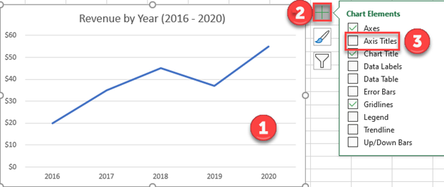
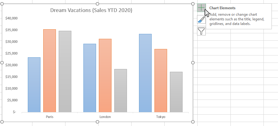
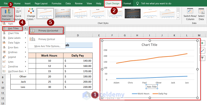
How to add data labels in excel to graph or chart (Step-by-Step) Jul 20, 2022 ... 1. Select a data series or a graph. · 2. Click Add Chart Element Chart Elements button > Data Labels in the upper right corner, close to the ... How to Add Data Labels to Graph or Chart on Microsoft Excel Mar 31, 2022 ... Want to know how to add data labels to graph in Microsoft Excel? This video will show you how to add data labels to graph in Excel. How to Make and Add Labels on a Graph in Excel Click the second button under the “Chart Layouts” section of the ribbon, which adds the labels to the chart. The location of this button varies depending on the ...

Adding chart labels in excel. trumpexcel.com › pie-chartHow to Make a PIE Chart in Excel (Easy Step-by-Step Guide) Related tutorial: How to Copy Chart (Graph) Format in Excel Formatting the Data Labels. Adding the data labels to a Pie chart is super easy. Right-click on any of the slices and then click on Add Data Labels. As soon as you do this. data labels would be added to each slice of the Pie chart. › make-pareto-chart-in-excelHow to Make Pareto Chart in Excel (with Easy Steps) Jul 25, 2022 · Steps to Make a Pareto Chart in Excel. I will use the following Sales Report to show you how to make a Pareto chart in Excel. In the dataset, the Product column consists of a list of product names. The Sales column consists of the corresponding sales amount for each product. Add or remove data labels in a chart - Microsoft Support Add data labels to a chart · Click the data series or chart. · In the upper right corner, next to the chart, click Add Chart Element · To change the location, ... superuser.com › questions › 188064Excel chart with two X-axes (horizontal), possible? - Super User A 3D column chart may accommodate the data, but not in a way that makes it at all intelligible. This would most likely be best as an XY Scatter chart, with two series: one using regular X values, the other using normalized X values, and both using the same Y values. After adding the secondary horizontal axis, delete the secondary vertical axis.

› pie-chart-excelHow to Create a Pie Chart in Excel | Smartsheet Aug 27, 2018 · To create a pie chart in Excel 2016, add your data set to a worksheet and highlight it. Then click the Insert tab, and click the dropdown menu next to the image of a pie chart. Select the chart type you want to use and the chosen chart will appear on the worksheet with the data you selected. How to add data labels and callouts to Microsoft Excel 365 charts? Step #1: After generating the chart in Excel, right-click anywhere within the chart and select Add labels. Note that you can also select the very handy option ... How to add data labels from different column in an Excel chart? Nov 18, 2021 ... How to add data labels from different column in an Excel chart? · 1. Right click the data series in the chart, and select Add Data Labels > Add ... › how-create-waterfall-chart-excelHow to Create a Waterfall Chart in Excel and PowerPoint Mar 04, 2016 · You’re almost finished. You just need to change the chart title and add data labels. Click the title, highlight the current content, and type in the desired title. To add labels, click on one of the columns, right-click, and select Add Data Labels from the list. Repeat this process for the other series.

Edit titles or data labels in a chart - Microsoft Support On the Layout tab, in the Labels group, click Data Labels, and then click the option that you want. Excel Ribbon Image. For additional data label options, click ... Adding Data Labels to Your Chart - Excel ribbon tips Aug 27, 2022 ... Activate the chart by clicking on it, if necessary. · Make sure the Layout tab of the ribbon is displayed. · Click the Data Labels tool. Excel ... Excel charts: add title, customize chart axis, legend and data labels Oct 5, 2022 ... To link an axis title, select it, then type an equal sign (=) in the formula bar, click on the cell you want to link the title to, and press the ... How to Make and Add Labels on a Graph in Excel Click the second button under the “Chart Layouts” section of the ribbon, which adds the labels to the chart. The location of this button varies depending on the ...

How to Create a Bar Chart With Labels Inside Bars in Excel

How to Add Data Labels to Graph or Chart on Microsoft Excel Mar 31, 2022 ... Want to know how to add data labels to graph in Microsoft Excel? This video will show you how to add data labels to graph in Excel.

How do i add Data labels on the Pareto Line for the Pareto ...

Excel Custom Chart Labels • My Online Training Hub

Custom data labels in a chart

How to add titles to Excel charts in a minute

How to Insert Axis Labels In An Excel Chart | Excelchat

Other Options for Chart Data Labels in PowerPoint 2011 for Mac

How to add live total labels to graphs and charts in Excel ...

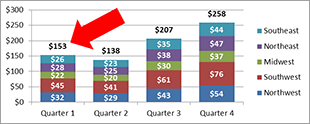
How to Add Totals to Stacked Charts for Readability - Excel ...

How To Show Or Hide Data Labels On MS Excel? | My Windows Hub

how to add data labels into Excel graphs — storytelling with data

Custom Data Labels with Colors and Symbols in Excel Charts ...

How to Add Two Data Labels in Excel Chart (with Easy Steps ...

Add label to Excel chart line • AuditExcel.co.za MS Excel ...

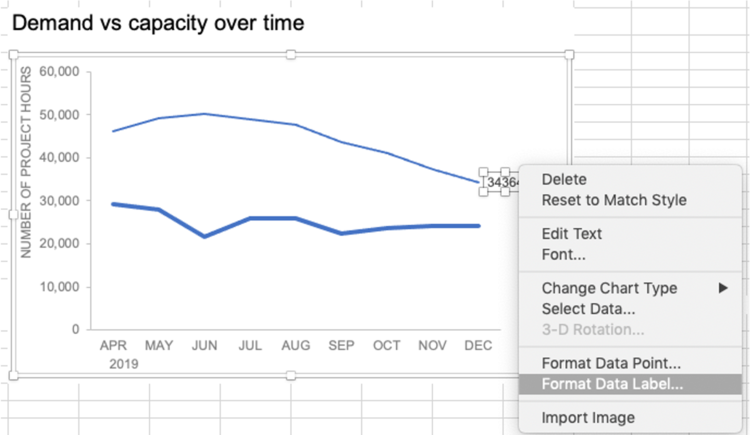
How to add or move data labels in Excel chart?

Add data labels and callouts to charts in Excel 365 ...

Change the format of data labels in a chart

Adding rich data labels to charts in Excel 2013 | Microsoft ...

How to add Axis Labels (X & Y) in Excel & Google Sheets ...

How to Add Axis Labels to a Chart in Excel - Business ...

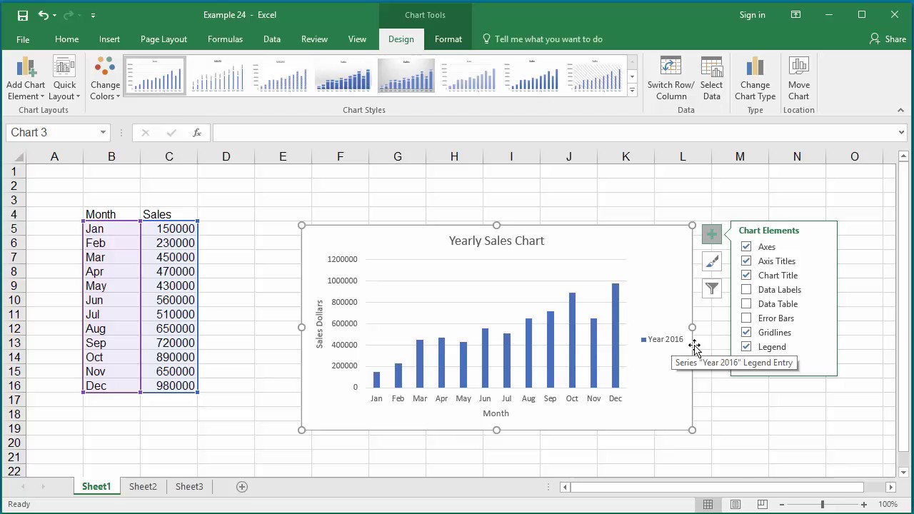
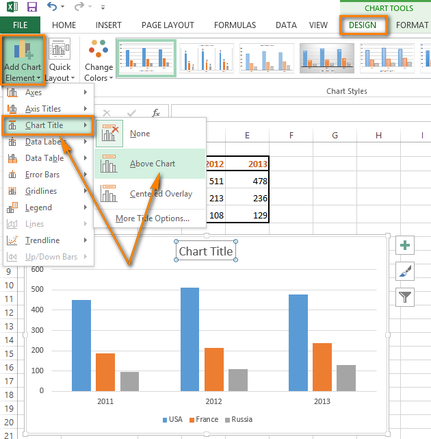
How to Change Elements of a Chart like Title, Axis Titles, Legend etc in Excel 2016

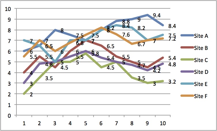
Directly Labeling Your Line Graphs | Depict Data Studio

Change the format of data labels in a chart

Dynamically Label Excel Chart Series Lines • My Online ...

How to Add and Remove Chart Elements in Excel

How to add axis labels in Excel - Quora

How to add total labels to stacked column chart in Excel?

Directly Labeling Excel Charts - PolicyViz

Enable or Disable Excel Data Labels at the click of a button ...

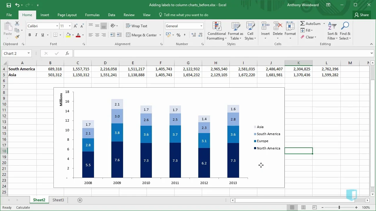
Adding Labels to Column Charts | Online Excel - KPMG Tax - Digital Now Course Training

Adding rich data labels to charts in Excel 2013 | Microsoft ...

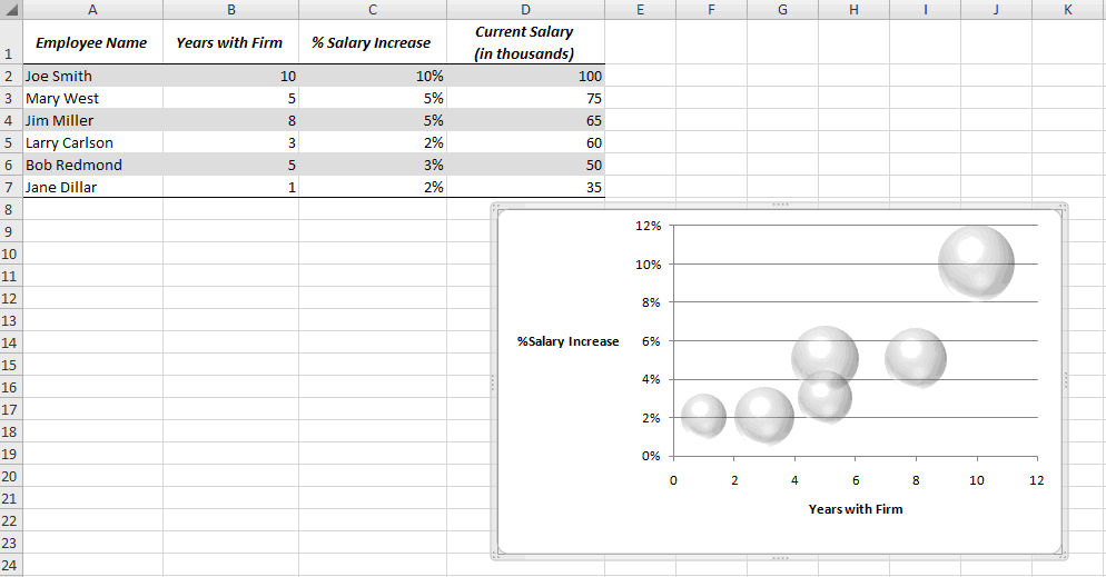
Add data labels to your Excel bubble charts | TechRepublic

Add or remove data labels in a chart

Chart Data Labels in PowerPoint 2013 for Windows

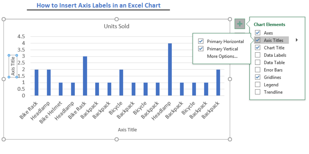
How to Insert Axis Labels In An Excel Chart | Excelchat

Directly Labeling Excel Charts - PolicyViz

Add Labels ON Your Bars

Apply Custom Data Labels to Charted Points - Peltier Tech

Add Percent Labels to a Bar Chart

Add a Data Callout Label to Charts in Excel 2013 – Software ...

Move and Align Chart Titles, Labels, Legends with the Arrow ...

Excel Add Axis Label on Mac | WPS Office Academy

How to Add X and Y Axis Labels in Excel (2 Easy Methods ...

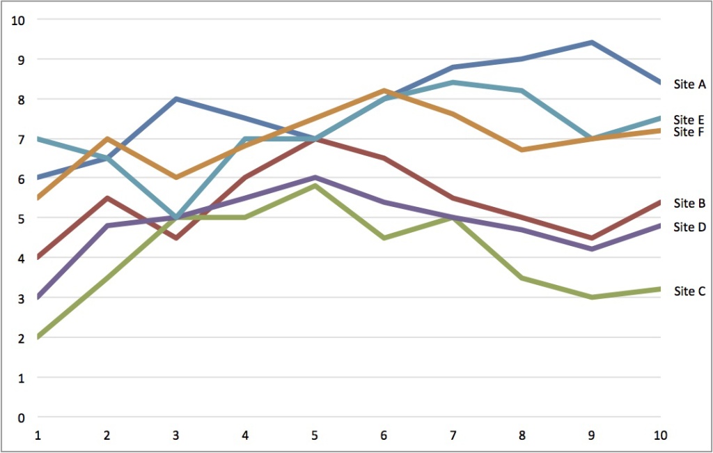
Directly Labeling Excel Charts - PolicyViz

Creating a chart with dynamic labels - Microsoft Excel 365

Your Custom Labels Online

45 adding chart labels in excel

Post a Comment for "45 adding chart labels in excel"

Menu Halaman Statis